Lab 7: Kalman Filter

See all the code I wrote on GitHub.

Step Response

To get the step response, I wrote some code that would drive the robot into a wall as fast as it could and stop if the robot get “close enough” to the wall to avoid damaging it. This code appears in my control loop, which looks very similar to how I implemented PID control.

Arduino (in loop()):

if (use_step_response) {
  motor_power = clip_motor_value(255);
  if (current_tof_front <= step_stop) {
    motor_power = 0;
    stop_motors(true);
  } else {
    move_forward(motor_power);
  }
  // log motor power, code omitted here
}

Jupyter Notebook:

bot = RobotControl(ble)
bot.stop_notify()
bot.set_motor_calibration(1.8)
bot.start_data_collection()
bot.start_step_response(400)
time.sleep(2.5)
bot.stop_step_response()
bot.stop()
bot.stop_data_collection()

The python code allows me to do a few things, like choose how close “close enough” is and change the motor calibration.

An aside: Programmable Calibration Factor

As I tried this, I ran into issues where my car would no longer drive straight. To avoid having to upload new code repeatedly, I created a command for this as well:

Arduino code (in handle_command()):

case SET_MOTOR_CALIB:
  success = robot_cmd.get_next_value(new_calib_factor);
  if (!success) return;
  motor_calib_factor = new_calib_factor;
  break;

Corresponding Python code (in RobotControl):

def set_motor_calibration(self, new_val):
  ble.send_command(CMD.SET_MOTOR_CALIB, new_val)

The calibration factor often depended on battery life, so it was helpful to be able to change it this way. This is also important for how the motor power is determined; to avoid driving in a non-straight line, the maximum motor power is clipped based on the calibration factor:

motor_power = clip_motor_value(255);
...
int clip_motor_value(float val_in) {
  if (val_in >= (255 / motor_calib_factor) ){
    return int(255 / motor_calib_factor);
  } else if (val_in <= MIN_POWER) {
    return 0;
  }
  return round(val_in);
}

Step Resonse Results

step response tof plot

step response vel plot

step response motor plot

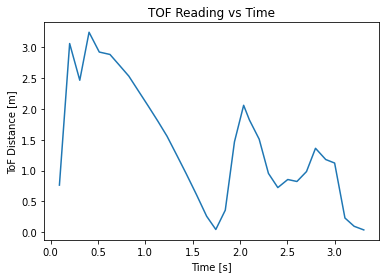
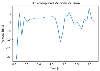
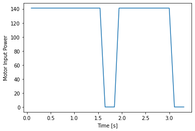
You may notice large spikes in the velocity plot. This is due to the measurement noise of the time of flight sensors, as the velocities are computed by computing the differences of adjacent elements in the time series.

Kalman Filter Output

See my code for this on GitHub

At first, when I used the parameters given in the lecture slides (scaled to meters instead of millimeters), my Kalman filter produced this plot:

sampling_rate=7.692307692307692
sigma_1=0.027735009811261455 m, sigma_2=0.027735009811261455 m/s, sigma_4=0.02 m
d=0.374251497005988, m=0.22754950399122473, rise time=1.4 s
Sigma_u:[[0.00076923 0.        ]
 [0.         0.00076923]]
Sigma_z:[[0.0004]]
A: [[ 0.          1.        ]
 [ 0.         -1.64470364]]
B: [[0.        ]
 [4.39464812]]
C: [[-1  0]]
mu_0: [[3.06]
 [0.  ]]
sigma_0: [[0.0363318 0.       ]
 [0.        0.       ]]

mediocre kalman filter plot

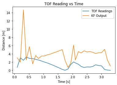
This plot doesn’t do a very good job of estimating where the true state is - I expected it to be closer to the ToF sensor readings, especially near the beginning. It also seems to change more quickly than it should be, which likely means I need to weigh the sensor values more than they presently are.

After tweaking the parameters, I was able to produce a better (but still not great) result:

sampling_rate=13.2
sigma_1=0.363318042491699 m, sigma_2=0.0363318042491699 m/s, sigma_4=0.025 m
d=0.374251497005988, m=0.22754950399122473, rise time=1.4 s
Sigma_u:[[0.132   0.     ]
 [0.      0.00132]]
Sigma_z:[[0.0004]]
A: [[ 0.          1.        ]
 [ 0.         -1.64470364]]
B: [[0.        ]
 [4.39464812]]
C: [[-1  0]]
mu_0: [[3.06]
 [0.  ]]
sigma_0: [[0.36331804 0.        ]
 [0.         0.        ]]

better kalman filter plot

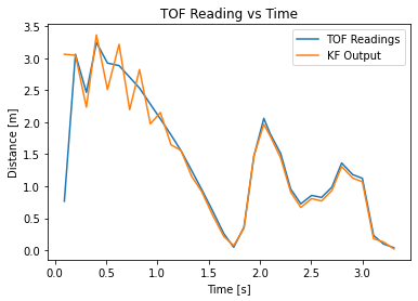
Each value in a covariance matrix (sigma) determines how much we trust either the model or the sensor, so we can use this to get some ballpark values:

The top left element of Sigma_u is the process noise in the position. I trust the sensor value to 0.3 meters.
The bottom right element of Sigma_u is the process noise in the velocity. I expect the model to do a much better job at predicting velocity, so I set it to something much smaller (about 0.04 m/s).
I know my sensor is noisy, so I set the measurment noise to 0.025 m (or 25 mm)
The rest of the computations follow from lecture.

This new plot is more consistent with my observed results - when trying this, the car drove in a mostly-straight line towards the wall, crashed (causing it to turn to a wall around a corner to approach it at an angle), and crashed into that wall as well. The new plot oscillates in the beginning though; I didn’t observe this, but I suspsect the oscillations come from the noisy sensor readings and how the car needed to overcome static friction in the beginning.

Kalman Filter Code

Most of the code is the same from lecture and lab handouts, but I made one minor change - in the given kf() code, I had to change the dimention of the identiy matrix because my state space is 2 by 1 (and not 3 by 1)

sampling_rate = len(tof_times) / 2.5 # ran for 2.5 seconds, see notebook code
sigma_1 = np.sqrt(0.1**2 * sampling_rate) # Trust in modeled position
sigma_2 = np.sqrt(0.01**2 * sampling_rate) # Trust in modeled speed
sigma_4 = 0.025 # measurement noise
sig_u=np.array([[sigma_1**2,0],[0,sigma_2**2]]) # u = dist from wall
sig_z=np.array([[sigma_4**2]]) # measurement noise

d = 1 / abs(steady_state_vel)
m = -d * rise_time / np.log(0.1)

A = np.array([[0,1], [0, -1*d/m]])
B = np.array([[0], [1/m]])
C = np.array([[-1,0]])

x = np.array([[tof_vals[1]],[0]])
delta_t = 1 / sampling_rate
A_d = np.eye(2) + delta_t * A
B_d = delta_t * B

def kf(mu_prev,sigma_prev,u,y):
    
    mu_p = A.dot(mu_prev) + B.dot(u) 
    sigma_p = A.dot(sigma_prev.dot(A.transpose())) + sig_u
    
    y_m = y-C.dot(mu_p)
    sigma_m = C.dot(sigma_p.dot(C.transpose())) + sig_z
    kkf_gain = sigma_p.dot(C.transpose().dot(np.linalg.inv(sigma_m)))

    mu = mu_p + kkf_gain.dot(y_m)    
    sigma=(np.eye(2)-kkf_gain.dot(C)).dot(sigma_p)

    return mu,sigma

After fixing an error with my code (I incorrectly scaled my motor input), I got this graph:

sampling_rate=13.2
sigma_1=0.363318042491699 m, sigma_2=0.0363318042491699 m/s, sigma_4=0.025 m
d=0.374251497005988, m=0.22754950399122473, rise time=1.4 s
Sigma_u:[[0.132   0.     ]
 [0.      0.00132]]
Sigma_z:[[0.000625]]
A: [[ 0.          1.        ]
 [ 0.         -1.64470364]]
B: [[0.        ]
 [4.39464812]]
C: [[-1  0]]
delta_t: 0.07575757575757576
A_d: [[1.         0.07575758]
 [0.         0.87540124]]
B_d: [[0.        ]
 [0.33292789]]
 mu_0: [[3.06]
 [0.  ]]
sigma_0: [[0.36331804 0.        ]
 [0.         0.        ]]

final kf try

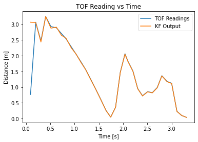
Although it looks like the Kalman Filter did little to the the position readings, the velocity plot seems smoother with the Kalman filter than without, although both still have large errors from the observed maximum speed of about 2 m/s.

kf velocity

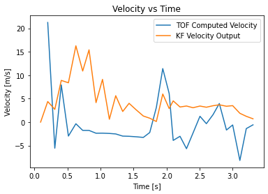
While I ran out of time to try the Kalman Filter on the robot (and would have wanted to tune it more in order for it to be useful), translating the Python code to Arduino wouldn’t be difficult:

#include <BasicLinearAlgebra.h>
using namespace BLA;

Matrix<2,2> A_d = {1, 0.07575758, 0, 0.87540124};
Matrix<2,1> B_d = {0, 0.33292789};
Matrix<2,1> C = {-1,0};
Matrix<2,2> sig_u = {0.132, 0, 0, 0,00132};
Matrix<1,1> sig_z = {0.000625};
Matrix<2,2> I_2 = {1,0,0,1};

Matrix<2,1> mu; Matrix<2,2> sigma; // to hold function results, multi return

void compute_kf(Matrix<2,1> mu_prev, Matrix<2,2> sigma_prev, Matrix<1,1> u, Matrix<1,1> y) {
  Matrix<2,1> mu_p = A_d*mu_prev + B_d*u
  Matrix<2,2> sigma_p = A*(sigma_prev*~A_d) + sig_u

  Matrix<1,1> y_m = y - (C*mu_p);
  Matrix<2,2> sigma_m = C*(sigma_p*~C) + sig_z;
  Matrix<2,1> kkf_gain = sigma_p * (~C*sigma_m.Inverse());

  mu = mu_p + kkf_gain*y_m;
  sigma = (I_2 - kkf_gain * C) * sigma_p;
}

ece4960-fast-robots