Lab 9: Mapping (real)

Click here to return to home page

Objective

Map a set-up series of walls and obstacles from multiple points in the lab.

Prelab

To make the map, I wanted to use my robot to spin in precise intervals and take sensor data to create a point cloud, much like how a radar creates one by knowing a series of angles and distances.

My plan was to do this:

1. Set up a PID controller to spin the robot 20 degrees, using the gyroscope to determine the angle
2. Read a ToF distance
3. Record the ToF distance and angle in an array on the robot
4. Repeat steps 1 through 3 until 1 revolution has been made
5. Send all the data back to a Jupyter notebook
6. Combine all the data into a map

But of course, this didn’t run smoothly…

Problems

Trying to get the robot to spin on its axis was difficult.. I had known this would happen, so I used my existing motor calibration command to change it on the Python side and send it to the robot. Experimentation revealed that the calibration value would range from 1.2 to 1.8 and change about once a day. Although this was an improvement, I also added tape to the wheels to allow them to slip easier.

PID control spun uncontrollably sometimes. To solve this, I realized that I made a sign error; if the signs are incorrect, the robot worsens its error instead of improves it because it spins in the opposite direction it needs to. This may be because of how the gyroscope is mounted, causing the code to appear “backwards”:

motor_power = pid_proportional * (pid_setpoint - pitch);

The robot’s gyroscope isn’t always an accurate way to determine heading. Although the robot would spin roughly the same amount per measurement, it would not always spin 20 degrees per measurement. To solve this, I added a parameter to change the time difference the robot uses to integrate gyrosocope angular velocity into position. This required some tuning, and this made some major improvements, but I also counted the number of motions needed to make a full revolution to clean up the data further.

offsets = {
  ...
  (0,3, 1): { # Start at (0,3), run 1
        "angle": (360/21) * np.pi / 180,
        "distance": (0, -0.5)
    },
  ...
}

The robot sometimes moves off its starting point before spinning. To compensate for this, I added a small parameter in the data cleanup code that allows me to make an offset to the spot the robot measures. That is, if the robot moved one tile to the left, I can input an offset that tells the measurements to behave as if they were taken from the floor tile the robot ended at instead of where the robot started.

offsets = {
  ...
  (-3,-2, 1): {
        "angle": (360/19) * np.pi / 180, # 19 "stops" per full rotation
        "distance": (0,-1)
    },
  ...
}

This is designed to work when the robot initially moves but doesn’t shift much while spinning, like in this video:

While this system works well, it’s not perfect; the robot can slide while it’s turning as well:

The ToF sensor is noisy at longer ranges. To mitigate this, I take the average of 3 consecutive readings from the same spot in order to make a plot.

// (P-controller code here)
} else if (abs(pitch - pid_setpoint) < 0.5) { // i.e. "close enough"
  stop_motors(true); 
  for (int i = 0; i < 3; i++){
    tof_meas = get_tof_measurement(distanceSensorTwo, true);
    // do other bookkeeping here
  }
  pid_setpoint += 20;
}

Data Processing

The data processing is somewhat sophisticated to combine all of the test points, so it’s helpful to see it step-by-step.

1. Watch the videos of the robot moving and construct a system of offsets:

   offsets = {
    (5,-3, 1): {
        "angle": 45 * np.pi / 180,
        "distance": (0,0),
    },
    (5,-3, 2): {
        "angle": (360/16) * np.pi / 180,
        "distance": (0,0)
    },
    etc...
   }
   

2. Load all the text files. I write my data in lists so I can simply use ast.literal_eval() to get the list from each line of text.

   for filename in glob.glob("data/*.txt"):
    with open(os.path.join(os.getcwd(), filename), 'r') as f:
        # Bookkeeping for start point and version
        new_data = dict()
        start = filename[5:-4].split("_")
        start_point = (int(start[0]), int(start[1]))
        version = int(start[2])
        new_data["start"] = start_point
        for line in f.readlines(): # read line-by-line to get all data
            if line.startswith("polar_points"):
                new_data["polar_points"] = ast.literal_eval(line[len("polar_points = "):])
            new_data["offset_polar_points"] = []
        version_key = (start_point[0], start_point[1], version)
        # Overwrite angles in data with observed angles in offsets dict
        if version_key in offsets.keys():
            for i, (r,_) in enumerate(new_data["polar_points"]):    
                new_data["offset_polar_points"].append((
                    r, 
                    i * offsets[version_key]["angle"], 
                    offsets[version_key]["distance"]
                ))
        data.append(new_data)
   

3. Convert to cartesan points.

   xy_points = []
   for d in data:
    (start_x, start_y) = d["start"]
    polar_points = d["offset_polar_points"]
    foot_to_mm = 304.8 # 304.8 in 1 foot (i.e. 1 lab tile side length)
    theta_offset = np.pi/2
    for (r,theta, dist) in polar_points:
        # Bot angles are measured clockwise-positive (while normal math measures the other way)
        # and bot angles start from 0 but are pi/2 in conventional math
        xy_points.append((
            r*np.cos(-1*theta + theta_offset) + start_x * foot_to_mm + dist[0] * foot_to_mm, 
            r*np.sin(-1*theta + theta_offset) + start_y * foot_to_mm + dist[1] * foot_to_mm
            ))
   

4. Make plots.

The Maps

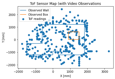
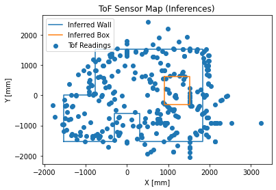
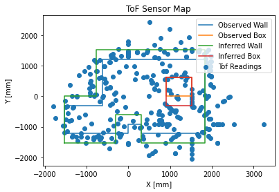
None of these maps are particularly clear; much of this is likely because of some combination of noise in the time of flight sensor, gyroscopic drift, and movement of the robot that isn’t perfectly along its axis. There may also be some added noise because of the walls themselves; some walls had a black felt lining, and some did not.

In an empty room, the robot would likely perform better; however, the noise from the ToF sensor and the gyroscope drift seem to be the limiting factors for accuracy. The angles drift by a few degrees per “20-degree” rotation, and the ToF sensor can sometimes have high-magnitude noise (like it did in the bottom right of the map).

Points

For the observed map:

wall_points = [
  (-5, -4), (0, -4), (0, -3), (1, -3), (1, -4), (6, -4), (6, 4), (-2, 4), (-2,-1), (-5,-1), (-5,-4)
]
box_points = [
  (3,2), (5,2), (5,0), (3,0), (3,2)
]

For the inferred map:

wall_points = [
  (-5, -5), (-1, -5), (-1, -2), (1, -2), (1, -5), (6, -5), (6, 5), (-2.5, 5), (-2.5,-0), (-5,-0), (-5,-5)
]
box_points = [
  (3,2), (5,2), (5,-1), (3,-1), (3,2)
]

These coordinates are given in feet, which happen to be the same length as the side of one tile. To convert these to distances in millimeters, multiply each number by f = 304.8 mm / tile